Troubleshooting¶

Technical Issues¶

Although every effort has been made to provide helpful error messages to correspond to every foreseeable issue, unfortunately not every issue is, in fact, foreseeable. This page is designed to help users troubleshoot should they run into issues not accompanied by a sufficiently helpful error message. Just because your transition path sampling shooting is aimless, doesn’t mean your troubleshooting has to be!

Issues running ATESA will fall into one of three categories, based on where in the pipeline the issue arises:

The local shell or the batch system
Amber
ATESA itself

A description of how to identify the category of error being encountered, and suggestions to resolve the issue, are provided. Further sections are provided for selected job types to facilitate troubleshooting in cases where the software appears to be functioning correctly, but the result is undesirable. If this page does not help you resolve your issue, please raise it on our GitHub page.

Issues with the local shell or the batch system¶

Errors encountered by these systems will appear in one of two places. If the shell encounters an error, it will be reported directly in the command line after ATESA is called. This likely indicates an issue with the installation of the software, or of Python itself. Command line errors will also arise if the batch system does not recognize the formatting of the batch files submitted by ATESA; double-check that your batch templates are of the correct format. Also, note that if ATESA is called from inside a batch job (as is recommended when performing many simulations), the command line output will be piped to the batch output file for that job.

Errors encountered by the batch system may also appear in batch output files for individual simulations, and in this case they will appear in the individual batch job output files in the working directory. These errors are likely to do with the formatting of the batch template files used by ATESA to create its job batch files. For example, if the user has removed the line in the batch template indicating the nodes to be assigned to the job on a Slurm system, ATESA will not complain (as omitting variables in the templates is supported in general), but the batch system will (because this particular variable is mandatory in Slurm). Other batch system errors include those not specific to ATESA, such as insufficient funds on the user account; to check whether a given error is of this type, try submitting a job that does not involve ATESA.

Issues with Amber¶

Amber has its own output file for each job, usually given by the suffix “.out” or “.mdout” in the working directory (note: ATESA may produce output files named with the “.out” suffix in this directory, as well.) If an error arises here, it likely indicates an issue with the formatting of the input coordinate or topology files, or else with the input file passed to Amber. Another common source of error when using certain QM/MM models is the absence of the necessary quantum mechanics files for the chosen level of theory. If these are missing they may need to be installed for you by a user with root access. ATESA has been tested in at least a limited capacity with Amber 12, 14, 16, and 18, but other versions are not guaranteed to be compatible.

Issues with ATESA¶

Sometimes, especially during aimless shooting, ATESA may hang, neither crashing nor apparently doing anything for a long time. In this case the easiest option is usually to restart the job with “restart = True” as appropriate.

Errors encountered by ATESA itself will be outputted into the command line in the event that the program has been called directly, or else into the batch output file in the event that it has been called in a batch job. Hopefully, most errors of this type will be self-explanatory. There may, however, be unforeseen errors that are not handled in a useful way. Errors of this sort could have to do with improperly installed dependencies, especially pytraj. One possible troubleshooting option is to retry the job with as many default settings as possible to see if the error persists — if it does not, add on custom settings one-by-one (starting with those you are least confident in) until the culprit is found.

If ATESA outputs an error message that confuses you, especially if it happens very early on in the job, double-check that the simulations that have been run so far (if there are any) appear to have behaved properly. For example, the error:

ValueError: must provie a filename or list of filenames or file pattern

is often the result of a failed simulation, usually because of a systemic issue in the way the model is set up. It may also arise when a necessary file has been errantly deleted. Regardless of the particular error, if everything seemed fine and then ATESA suddenly crashed, often simply resubmitting the job (with restart = True, as appropriate) will fix it.

Another common issue is:

EOFError: Ran out of input

while trying to open the restart pickle file (“restart.pkl”). This occurs because the restart file has been errantly emptied due to an interrupted write attempt. ATESA automatically generates a backup file called “restart.pkl.bak” in the working directory, so if you get this error, simply copy the backup file over the empty original.

Repeated “errors” with messages like these while running simulations are normal and not an issue so long as ATESA continues to run:

Internal Error: Global index 0 is out of range.
Error: NetCDF file has no frames.
Error: Could not set up '<trajectory file>' for reading.

Although the user is of course permitted under the license to attempt to debug the code themselves (and to use the modified code in whatever manner they see fit), no one finds it easy to read someone else’s code. If you encounter an issue with ATESA that you cannot resolve, I encourage you to raise an issue on our GitHub page. And if you encounter an error that you did resolve by modifying the code, please submit a pull request so that everyone can benefit!

Job Type-Specific Issues¶

This section concerns issues that may arise in individual job types when the code is apparently functioning properly, but the results are in some way not satisfactory. Not every possible issue can be mentioned here, so if you come across something that’s stumped you and isn’t addressed on this page, please raise an issue on our GitHub page with the “question” and/or “help wanted” tags.

Aimless Shooting¶

Barring technical issues, the only problem you might experience during aimless shooting is very low acceptance ratios. The acceptance ratio for each thread represents the ratio of shooting moves that have been “accepted” (recall that this means that the combined foreward and backward trajectories connect one stable state to the other) to the total number of shooting moves in that thread so far. The acceptance ratio is sensitive to many factors, including the initial coordinates, the min_dt and max_dt configuration file settings, and the underlying energetic landscape, but in general a “good” acceptance ratio is somewhere in the range of 10-to-40%. The efficiency of aimless shooting in sampling the state space around the separatrix is directly tied to the acceptance ratio, so in general it is important to be getting an acceptable value. While higher acceptance ratio values are not a problem, they may indicate that your sampling is too conservative (differences between adjacent shooting points are too small), which also negatively impacts sampling efficiency.

A chronically low acceptance ratio during aimless shooting, even across many degenerate threads or slightly different input coordinate files, probably indicates that your initial coordinates are not as close to the reaction separatrix as you might have hoped. Even if they are very close, an extremely steep energetic landscape makes aimless shooting difficult, and depending on the context of your study may indicate an incorrect putative reaction mechanism. You should also consider making the max_dt and/or min_dt settings smaller; although larger values can explore phase space more efficiently, it also increases the risk of a thread straying too far from the separatrix and being unable to climb back up, resulting in poorer acceptance ratios after that step. This effect can be mitigated by setting always_new to “True” (which is the default).

If you are getting zero acceptance despite the simulations themselves looks reasonable, you should interpret it to mean that your initial coordinates are too far from the separatrix to be acceptable. If you obtained your initial coordinates through some means other than ATESA’s jobtype = find_ts option, you should give that a try, as it will only ever provide coordinates with non-zero acceptance ratios (and provide custom advice if it is unable to do so). Otherwise, you’ll have to look to whatever means you’re using to obtain your initial coordinates.

Finally, if simulations seem to be going fine but are simply taking a very long time, the issue is probably with the setup of individual jobs. As always when running a new model on a high performance cluster, you should first run a series of short jobs to assess how your simulation speed scales with the resources allocated. Keep in mind that certain settings are much more computationally expensive (and thus slow), such as large quantum mechanics regions. Also ensure that you have allocated sufficient memory for each job and for ATESA itself; at least a few gigabytes is safe.

Committor Analysis¶

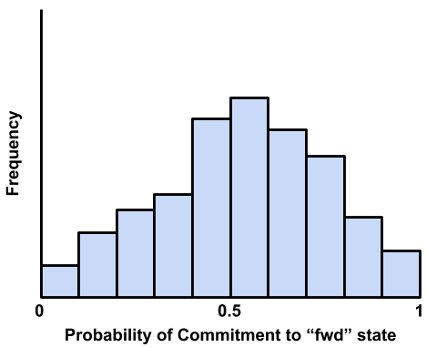
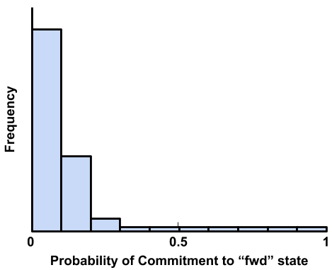
The “ideal” committor analysis result is a perfectly narrow peak of exactly 50% probability of going to each stable state. In practice however, the best result we can hope for is a roughly gaussian distribution peaked somewhere close to 50%, and a roughly flat distribution is also generally acceptable. The rest of this section will be organized in terms of other possible distributions with advice about how to interpret them, and then ending with some examples of real published committor analysis results.

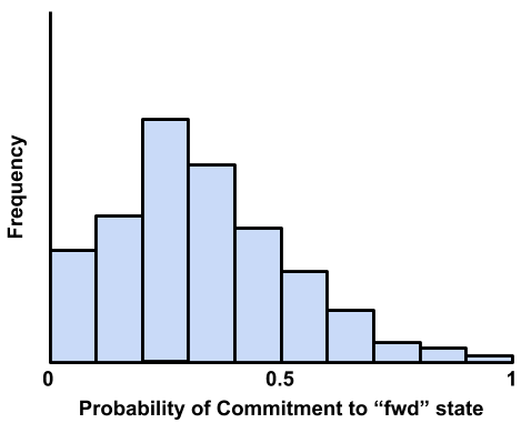
This is an example of an excellent committor analysis result. The model used to arrive at this result appears to be very strong. That the peak is not quite at 0.5 is of little consequence, and in fact to be expected when attempting to describe very high-dimensional systems with a relatively low-dimensional model.

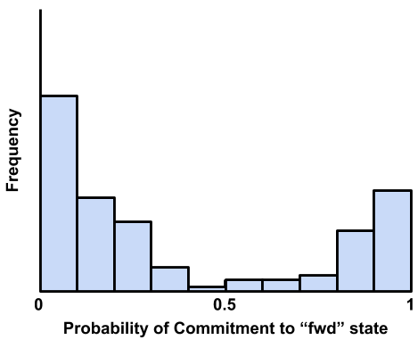
A common poor committor analysis result, the distribution is bimodal at or near the edges. This happens when the model was built along a dimensional projection that causes shooting points on opposite sides of the actual separatrix to look close together. Usually it means that one or more key dimensions has been omitted from the list of candidate CVs, so add as many as you can imagine might be important and run aimless shooting with resample = True to resample the shooting points with your new CVs before attempting likelihood maximization and committor analysis again.

The distribution is roughly gaussian, but centered far from 50%. This is another common result that arises when there’s simply not enough data from aimless shooting to arrive at a strong model through likelihood maximization. If the peak isn’t right along an edge (0 or 1) then this result is still fairly strong, but if you want to improve it, simply collecting more data or using a higher-dimensional reaction coordinate may help.

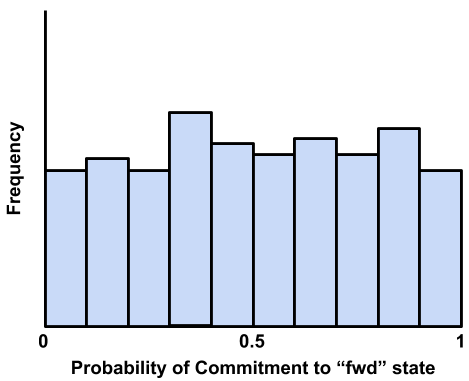
A roughly flat distribution, this result can arise either from insufficient sampling during aimless shooting or committor analysis, missing candidate dimensions, or the use of a lower-dimensional model than is truly appropriate for the system. Similarly to the previous example, this is still a reasonably strong result and may indicate a strong enough model, depending on your purposes.

All or nearly all of the simulations are grouped along one edge (either one). This should be a rare result, and is the only one here that represents a fundamental failure somewhere in the workflow. The underlying cause is either: (a) that the settings or other important features of the simulations or ATESA have changed significantly between aimless shooting and committor analysis (for example, a different quantum mechanics model, or a change in the definition of the commitment basins); or (b) that the aimless shooting data has been misinterpreted in some way, due to some unnoticed error. If after carefully verifying that the settings have not changed (remember to check the simulation input files, batch file templates, and ATESA configuration files) you still cannot find the source of this error, please raise an issue on our GitHub page with the “bug” label. Please also be sure to include a thorough description of your problem and attach the files “settings.pkl” and “restart.pkl” from the aimless shooting working directory.

Here are some examples of real committor analysis results in published manuscripts. Though none are perfect, all of these results were deemed acceptable within the context of their work by their authors and passed peer review.

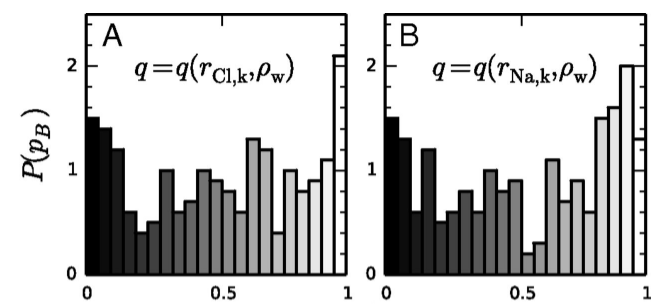
Joswiak, M. N., Doherty, M. F., & Peters, B. (2018). Ion dissolution mechanism and kinetics at kink sites on NaCl surfaces. Proceedings of the National Academy of Sciences, 115(4), 656–661. https://doi.org/10.1073/pnas.1713452115

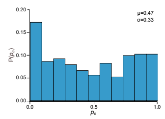
Mayes, H. B., Knott, B. C., Crowley, M. F., Broadbelt, L. J., Ståhlberg, J., & Beckham, G. T. (2016). Who’s on base? Revealing the catalytic mechanism of inverting Family 6 glycoside hydrolase. Chemical Science, 5955–5968. https://doi.org/10.1039/C6SC00571C

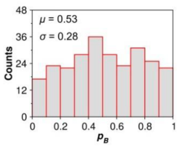
Silveira, R. L., Knott, B. C., Pereira, C. S., Crowley, M. F., Skaf, M. S., & Beckham, G. T. (2021). Transition Path Sampling Study of the Feruloyl Esterase Mechanism. Journal of Physical Chemistry B, 125(8), 2018–2030. https://doi.org/10.1021/acs.jpcb.0c09725

Umbrella Sampling¶

Umbrella sampling is a powerful tool for efficiently evaluating the free energy profile along a chosen reaction coordinate. However, as with all restrained simulations methods the simulations may not behave as expected, leading to errant results. In this section we will describe a few types of errors commonly encountered during umbrella sampling and suggest solutions. Note that this section assumes that the simulations and code are running without error, and that the issue is instead with the data itself.

The standard workflow when analyzing umbrella sampling data with ATESA is to run mbar.py with the -i flag pointing to the umbrella sampling working directory. Before analyzing the data, this script returns two “diagnostic” plots to help the user ensure that the data is sound (these plots are returned numerically instead of graphically in the output file (default name mbar.out) if the shell does not support producing graphs directly, in which case you can plot them yourself). The first is a histogram and the second is a “mean value” plot.

The Histogram

The histogram is actually composed of many individual histogram plots, one for each unique window center in the data. The purpose of the histogram is to visually ensure that there are no gaps in the data (that is, that there are no large regions between histograms where no sampling has occurred) and that the sampling is roughly even (that is, that all of the peaks are roughly at the same height, though there will be some natural variation).

If there are gaps, the solution may simply be to run additional simulations with the same restraint weight centered in the under-sampled region(s). Keep in mind that there is no need for the sampling windows to be evenly spaced. Alternatively, if the gaps are caused by restrained simulations in those regions falling away from them, you should either redo umbrella sampling with increased the restraint weights (which may necessitate more tightly packed windows) and/or with What is Pathway-Restrained Umbrella Sampling? enabled.

If there are under-sampled regions, you should investigate the root cause by looking to the simulations in those regions themselves. One potential source of this issue in reaction models is poor quantum mechanical convergence. Resolving this issue is highly system-specific and lies outside the scope of this document, but note that in some cases it may be alleviated by adding a small electronic temperature to the simulations.
The Mean Value Plot

The second plot is a line plot depicting the difference between the mean value of the sampling data in each window and that window’s restraint center on the vertical axis, versus the window restraint center on the horizontal axis. If there are multiple simulations located at the same window center (and there ought to be; by default there are five), these will be averaged together.

The ideal mean value plot should be a smooth sinusoid passing through the value of zero on the vertical axis at three points: near the leftward extreme, near the middle, and near the rightward extreme. These correspond to the regions of the free energy profile with zero slope at one stable state, the transition state, and the other stable state, respectively. If either of the extrema do not pass through zero, further umbrella sampling windows should be added on the corresponding end until zero (and ideally, a little bit beyond) is reached.

The other issue visible on this plot is unsmoothness. Unsmoothness includes both incongruently large error bars compared to other windows, or an abrupt discontinuity between adjacent points on the plot. This is usually caused by sampling of two or more significantly different regions of state space with similar reaction coordinate values. Depending on the underlying cause of this issue, it may be solvable using ATESA’s pathway-restrained umbrella sampling feature (see What is Pathway-Restrained Umbrella Sampling? for details). It can also be improved in many cases by using an alternate reaction coordinate, especially a higher-dimensional one where any further dimensions are largely orthogonal to those already included.

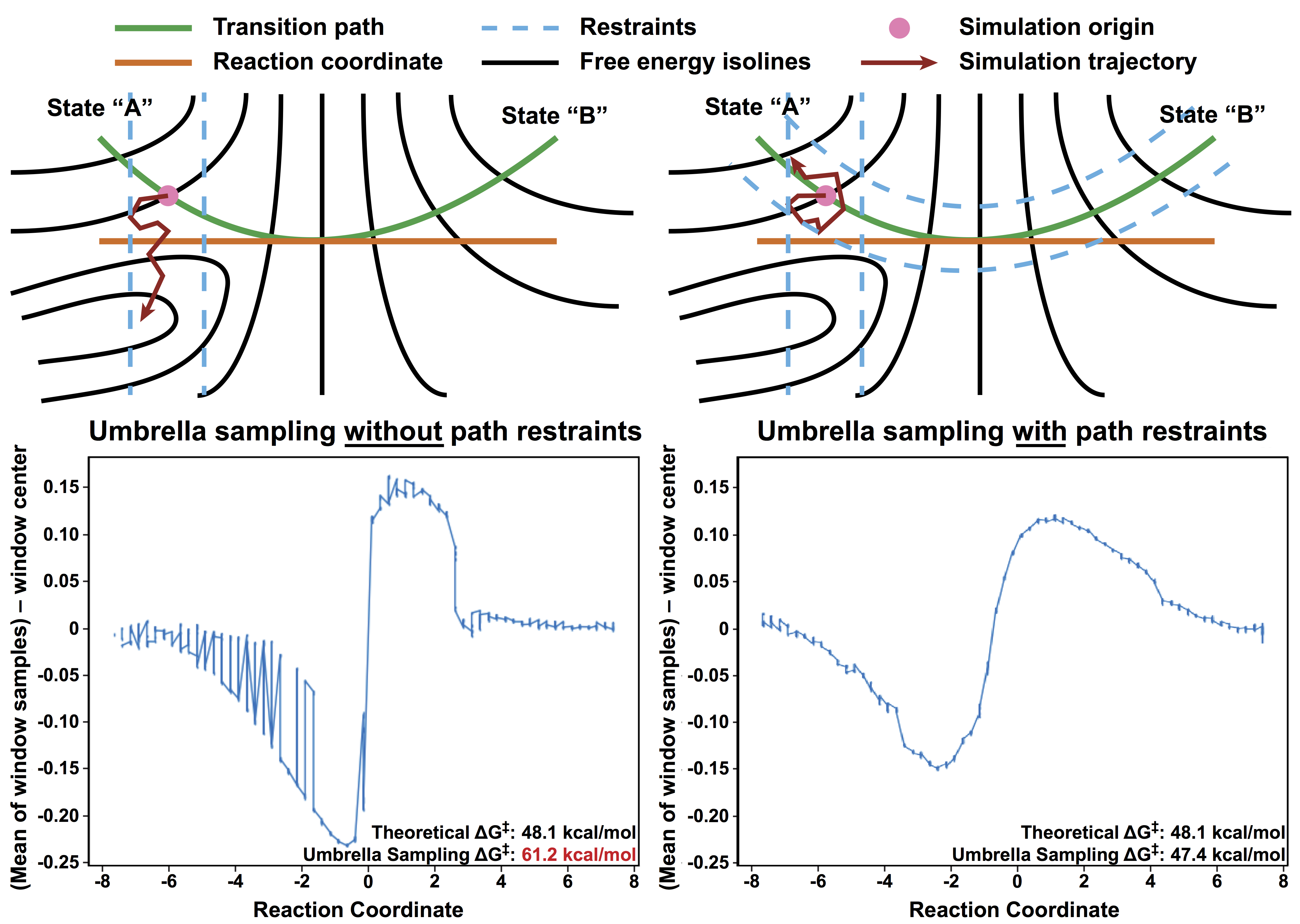
An example of the sort of error that can necessitate pathway-restrained umbrella sampling. (a) Two energetically distinct structures with identical reaction coordinate values for the example system (see Example Study). This is the sort of error that causes unsmoothness within a single window. (b) Examples of mean value plots. The mean value plot on the left is unsmooth, but application of pathway restraints results in the much-improved plot on the right.